MIT 6.S183 Homeworks
Homeworks in MIT 6.S183: A Practical Introduction to Diffusion Models
Problem Set1
Question1
a. Prove that for any distribution over random variables \(X\) and \(Y\) we have
\[\arg\min_f \mathbb{E}_{x,y} \big[ \|f(y) - x\|^2 \big] = \mathbb{E}[x \vert y].\]Hint: Solve the optimization problem pointwise for fixed \(y\).
Proof
With the law of total expectation, we have
\[\mathbb{E} \big[ \|f(y) - x\|^2 \big] = \mathbb{E}_Y \bigg[ \mathbb{E}_X \big[ \|f(y) - x\|^2 \vert Y = y \big] \bigg]\]For any fixed \(y\), \(f(y)\) is nothing but a constant. Let \(c = f(y)\), the inner expectation could be expressed as
\[\begin{aligned} \mathbb{E}_X \big[ \|f(y) - x\|^2 \vert Y = y \big] &= \mathbb{E}_X [ \| c - x\|^2 \vert Y=y ] \\ &= \mathbb{E}_X [ c^2 - 2 c x + x^2 \vert Y=y ] \\ &= c^2 - 2c \mathbb{E} [X \vert Y=y] + \mathbb{E} [X^2 \vert Y=y] \end{aligned}\]Obviously, the minimizer of \(c\) is
\[c^* = f(y) = \mathbb{E} [X \vert Y=y]\]This is also known as the MMSE estimator.∎
b. Let \(\mu\) be the density function of a data distribution, so that \(\mu(x_0) \geq 0\) for all \(x_0 \in \mathbb{R}^n\) and \(\int_{\mathbb{R}^n} \mu(x_0) \mathrm{d} x_0 = 1\). Consider the following loss function for fixed \(\sigma\).
\[\mathcal{L}_{\sigma}(\epsilon_{\sigma}) = \mathbb{E}_{x_0 \sim \mu, \epsilon \sim N(0, I_n)} \left[ \|\epsilon_{\sigma}(x_0 + \sigma \epsilon) - \epsilon\|^2 \right]\]Write down the exact minimizer \(\epsilon_{\sigma}^*(x_{\sigma})\) in terms of the data distribution \(\mu(x_0)\) and input \(x_{\sigma}\).
Hint: use part a, Bayes' rule, as well as the probability density function of \(N(x_0, \sigma^2 I_n)\).
Solve
From part a, the minimizer of \(\epsilon_{\sigma}\) has the closed form
\[\epsilon_{\sigma}^*(x_{\sigma}) = \mathbb{E}[\epsilon \vert x_{\sigma} = x_0 + \sigma \epsilon]\]Then, with the forward diffusion process, the added noise could be expressed as
\[\epsilon = \frac{x_\sigma - x_0}{\sigma}\]As a result, the minimizer is
\[\begin{aligned} \epsilon_{\sigma}^*(x_{\sigma}) &= \mathbb{E} \bigg[\frac{x_\sigma - x_0}{\sigma} \bigg\vert x_{\sigma} \bigg] \\ &= \frac{1}{\sigma} \big( x_\sigma - \mathbb{E}[x_0 \vert x_\sigma] \big) \end{aligned}\]Now we need to solve the posterior expectation \(\mathbb{E}[x_0 \vert x_\sigma]\). To start with, the posterior probability density function \(p(x_0 \vert x_\sigma)\) could be derived with the Baye's rule:
\[\begin{aligned} p(x_0 \vert x_\sigma) &= \frac{p(x_\sigma \vert x_0) p(x_0)}{p(x_\sigma)} \\ &= \frac{p(x_\sigma \vert x_0) p(x_0)}{\int p(x_\sigma \vert x_0) p(x_0) \mathrm{d} x_0} \\ &= \frac{p(x_\sigma \vert x_0) \mu(x_0)}{\int p(x_\sigma \vert x_0) \mu(x_0) \mathrm{d} x_0} \end{aligned}\]Since \(x_\sigma \vert x_0 \sim N(x_0, \sigma^2 I_n)\), the posterior probability density function becomes
\[p(x_0 \vert x_\sigma) =\frac{\mu(x_0) \exp{ \bigg( -\frac{\| x_\sigma - x_0 \|^2}{2\sigma^2} \bigg)}}{\int \mu(x_0) \exp{ \bigg( -\frac{\| x_\sigma - x_0 \|^2}{2\sigma^2} \bigg)} \mathrm{d} x_0}\]Now, the posterior expectation is given by
\[\mathbb{E}[x_0 \vert x_\sigma] = \frac{\int x_0 \cdot \mu(x_0) \exp{ \bigg( -\frac{\| x_\sigma - x_0 \|^2}{2\sigma^2} \bigg)} \mathrm{d} x_0}{\int \mu(x_0) \exp{ \bigg( -\frac{\| x_\sigma - x_0 \|^2}{2\sigma^2} \bigg)} \mathrm{d} x_0}\]To sum up, the minimizer has the closed form
\[\begin{aligned} \epsilon_{\sigma}^*(x_{\sigma}) &= \frac{1}{\sigma} \big( x_\sigma - \mathbb{E}[x_0 \vert x_\sigma] \big) \\ &= \frac{\int (x_\sigma - x_0) \cdot \mu(x_0) \exp{ ( -\| x_\sigma - x_0 \|^2/{2\sigma^2} )} \mathrm{d} x_0}{\sigma \int \mu(x_0) \exp{ ( -\| x_\sigma - x_0 \|^2/{2\sigma^2} )} \mathrm{d} x_0} \end{aligned}\]∎
c. Let \(x_0\) be a random variable distributed according to some continuous density \(p_0(x)\). Define \(x_t := x_0 + \sigma(t)\epsilon\) for some function \(\sigma : [0, 1] \rightarrow \mathbb{R}_{\geq 0}\) and let \(p_t(x)\) be the probability density associated with \(x_t\). Show that \(v(x, t) = \mathbb{E} \bigg[\frac{d\sigma(t)}{dt} \mid x_t = x \bigg]\) and \(p_t(x)\) satisfy the transport equation governing the evolution of the density \(p_t\) subject to a velocity field \(v\):
\[\partial_t p_t(x) + \nabla \cdot (v(x, t) p_t(x)) = 0\]Hint: Consider the time derivative of the characteristic function \(g(t, k) = \mathbb{E}[e^{ik \cdot x_t}]\). You may also use the fact from Fourier analysis that
\[\int e^{ik \cdot x} \nabla \cdot f(x) \mathrm{d} x = -ik \cdot \int e^{ik \cdot x} f(x) \mathrm{d} x\]and, for continuous functions \(f\) and \(g\), \(\int e^{ik \cdot x} f(x) \mathrm{d} x = \int e^{ik \cdot x} g(x) \mathrm{d} x\) iff \(f = g\).
Proof
Take the time derivative of the characteristic function
\[\begin{aligned} \partial_t \tilde{p}_t (k) &= \frac{\partial}{\partial t} \mathbb{E}[e^{ik \cdot x_t}] \\ &= \mathbb{E} \bigg[\frac{\partial}{\partial t} e^{ik \cdot x_t} \bigg] \\ &= \mathbb{E} [ e^{ik \cdot x_t} \cdot ik \cdot \partial_t x_t ] \end{aligned}\]Consider the forward diffusion process
\[\partial_t x_t = \partial_t \big(x_0 + \sigma (t) \epsilon \big) = \sigma' (t) \epsilon\]Then, the time derivative part gives
\[\partial_t \tilde{p}_t (k) = ik \ \mathbb{E} [ e^{ik \cdot x_t} \cdot \sigma' (t) \cdot \epsilon ]\]Now, with the law of total expectation, the expectation term could be expressed as
\[\begin{aligned} \mathbb{E} [ e^{ik \cdot x_t} \cdot \sigma' (t) \cdot \epsilon ] &=\mathbb{E} \big[ \mathbb{E} [ e^{ik \cdot x_t} \cdot \sigma' (t) \cdot \epsilon \vert x_t = x ] \big] \\ &= \mathbb{E} [ e^{ik \cdot x} \cdot \mathbb{E} [ \sigma' (t) \cdot \epsilon \vert x_t = x ] ] \\ &= \mathbb{E} [ e^{ik \cdot x} \cdot v(x, t) ] \end{aligned}\]As a result,
\[\partial_t \tilde{p}_t (k) = ik \cdot \mathbb{E} [ e^{ik \cdot x} \cdot v(x, t) ]\]Now consider the transport equation. Use Fourier transform on the LHS,
\[\begin{aligned} \text{LHS} &= \int e^{ik \cdot x} \ \partial_t p_t(x) \ \mathrm{d} x + \int e^{ik \cdot x} \ \nabla \cdot (v(x, t) p_t(x)) \ \mathrm{d} x \\ &= \partial_t \tilde{p}_t (k) - ik \int e^{ik \cdot x} \ v(x, t) \ p_t(x) \ \mathrm{d} x \\ &= \partial_t \tilde{p}_t (k) - ik \cdot \mathbb{E} [ e^{ik \cdot x} \cdot v(x, t) ] \\ &= 0 \end{aligned}\]Finally, we have proved the transport equation
\[\partial_t p_t(x) + \nabla \cdot (v(x, t) p_t(x)) = 0\]∎
Question2
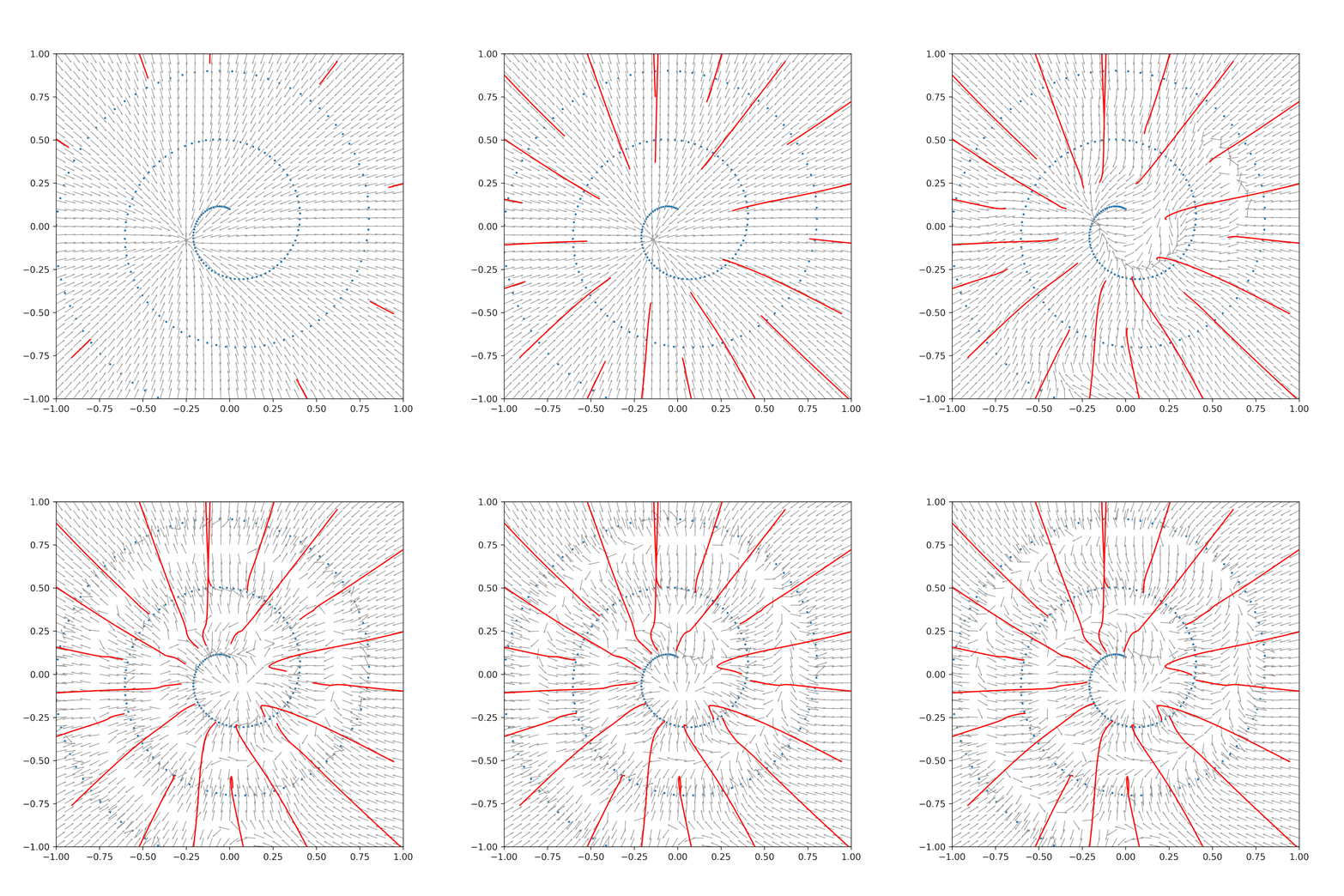
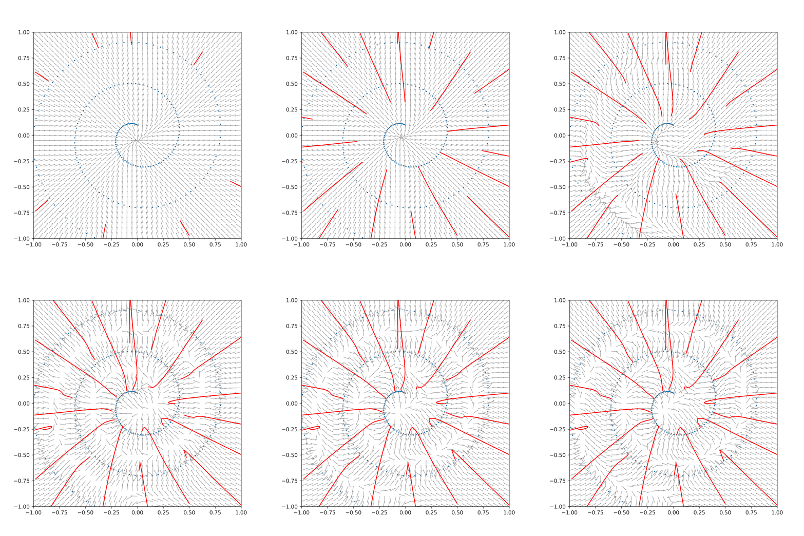
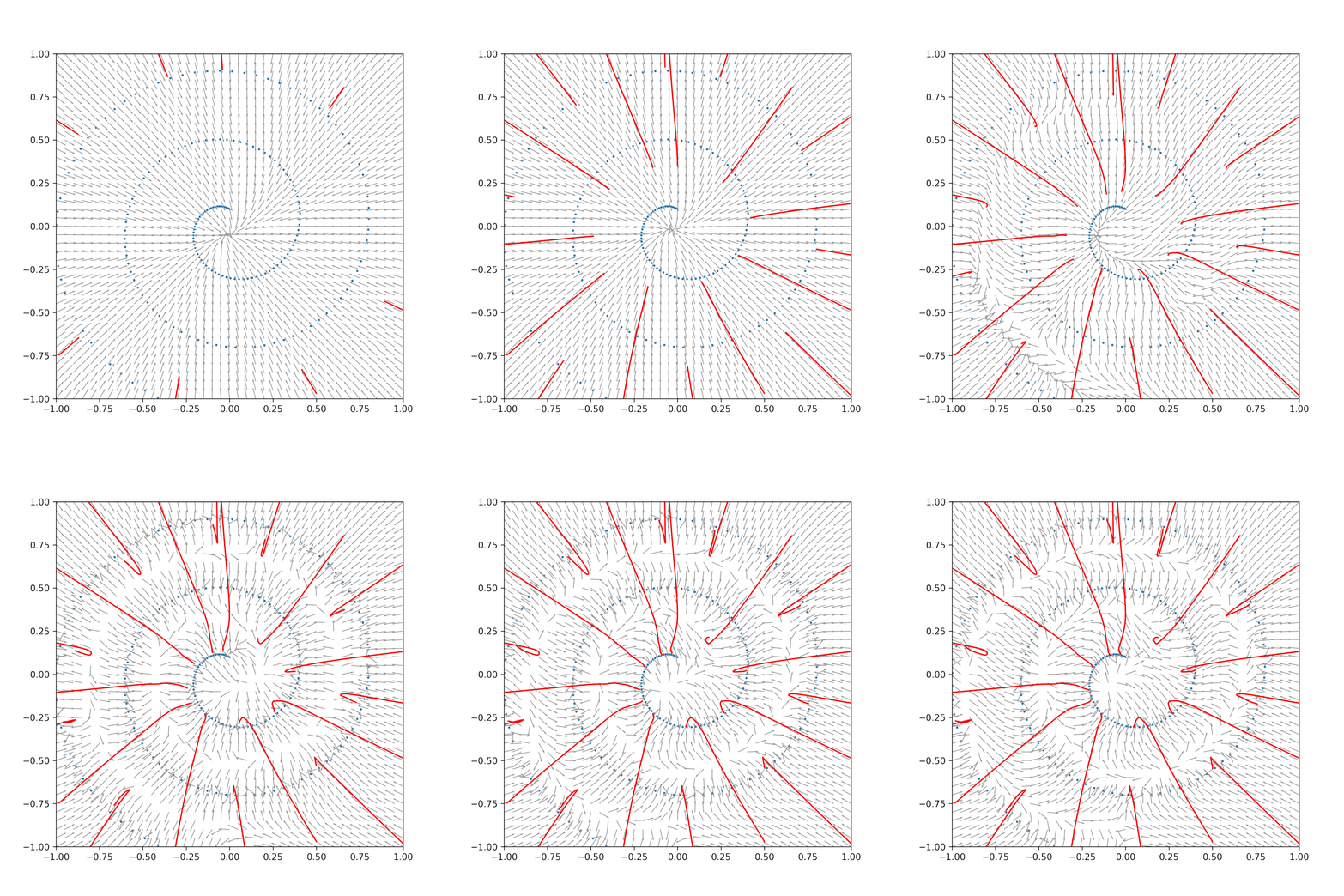
DDIM Sampler
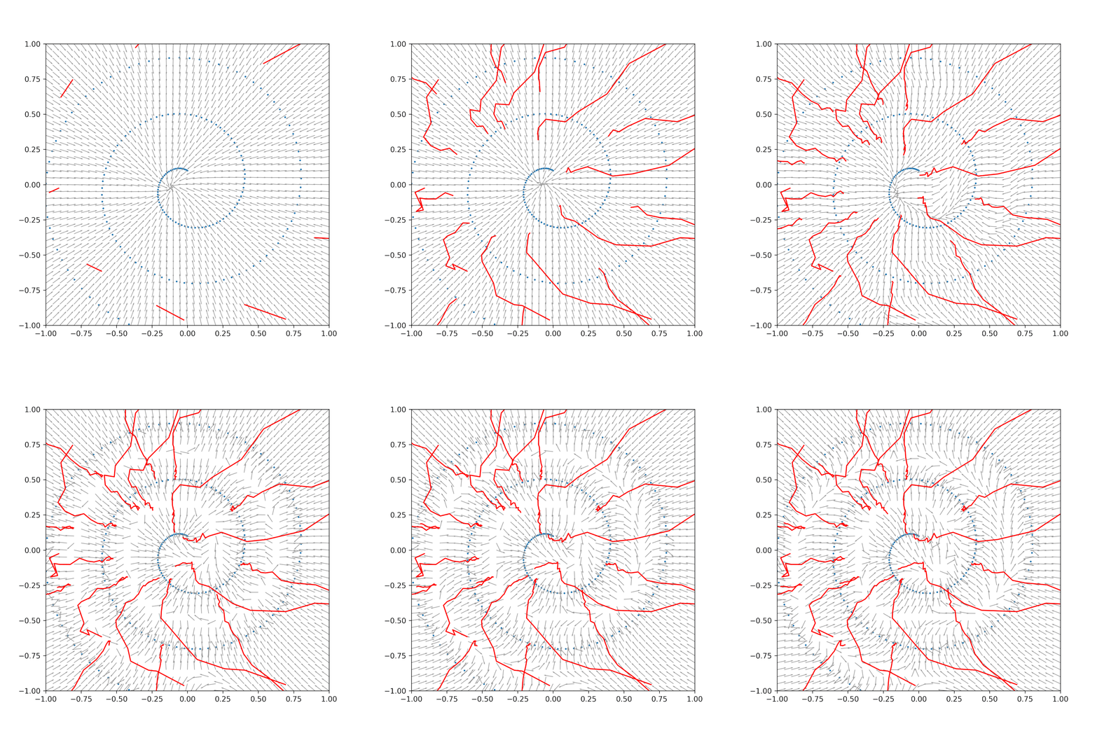
DDPM Sampler
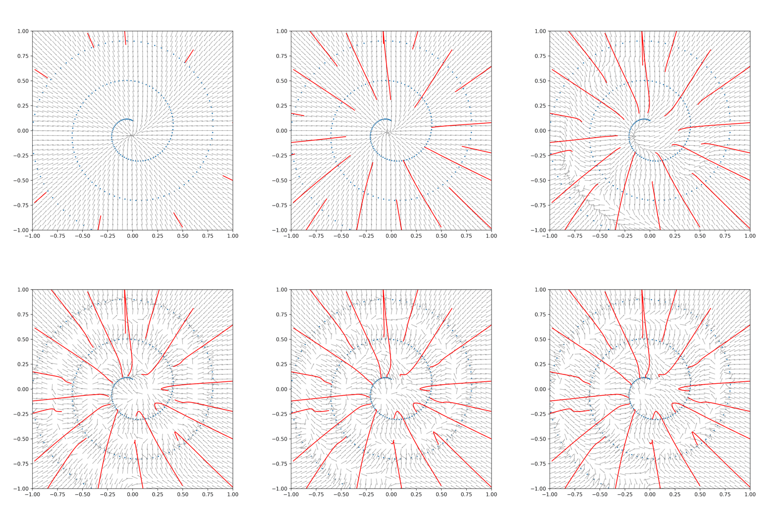
Accelerated Sampler
Implement accelerated sampler according to Interpreting and Improving Diffusion Models from an Optimization Perspective.
Problem Set2
Image Interpolation with Diffusion
Building in a futuristic city, oil painting, ghibli inspired, high resolution → House in the woods, oil painting, ghibli inspired, high resolution

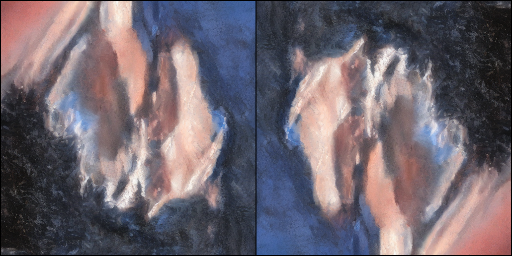
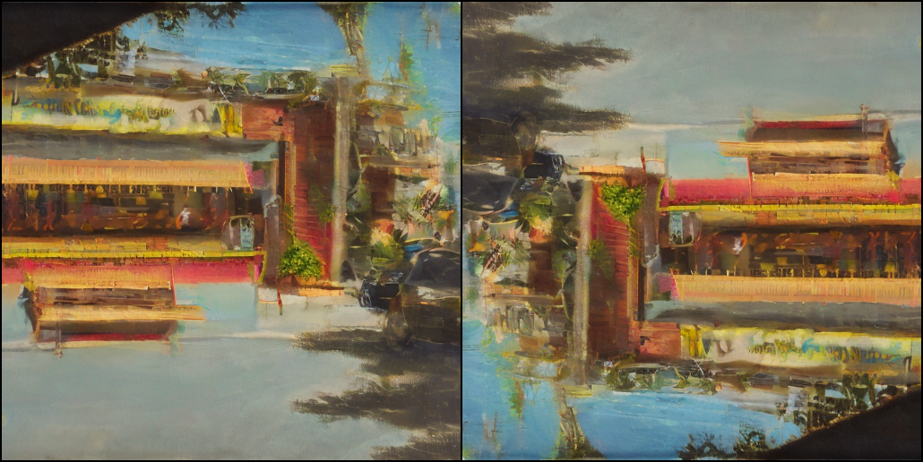
Visual Illusions with Diffusion
A painting of a snowy mountain → A painting of a horse
An oil painting of a restaurant → An oil painting of a palace
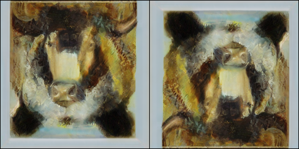
A painting of a bull → A painting of a bear